
- April 4, 2024
- By Pablo Diego Rosell
- Rosan International
I was recently asked by some colleagues to demonstrate the usefulness of Multilevel Regression and Post-stratification (MRP) for small area estimation. I initially resorted to the classics (Gelman et al.), pointing out the efficiency of pooling data to estimate regressors across small areas, then applying census data or other external sources of ground truth to post-stratify these regression estimates to population counts in each small area. However my colleagues are not easily impressed by big words and famous names , so I had to build a small simulation to demonstrate these principles.
I present below an abridged version of this simulation, focusing on three scenarios:
1) Baseline: Individual-level variance but no aggregate-level variance.
2) MRP-favorable: Individual-level and aggregate-level variance correlated with an external aggregate-area indicator.
3) MRP Neutral: Individual-level and aggregate-level variance uncorrelated with an external aggregate-area indicator.
The purpose of these simulation is to evaluate how MRP would perform in terms of bias and variance relative to estimating means directly from the national average (fixed means) or from the sample (sample means).
- 1 Setup Simulation
- 2 Simulation Scenarios
- 3 Simulate Population Data 1: No small_area-level variance
- 4 Simulate Population Data 2: small_area-level attitude variance correlated with income
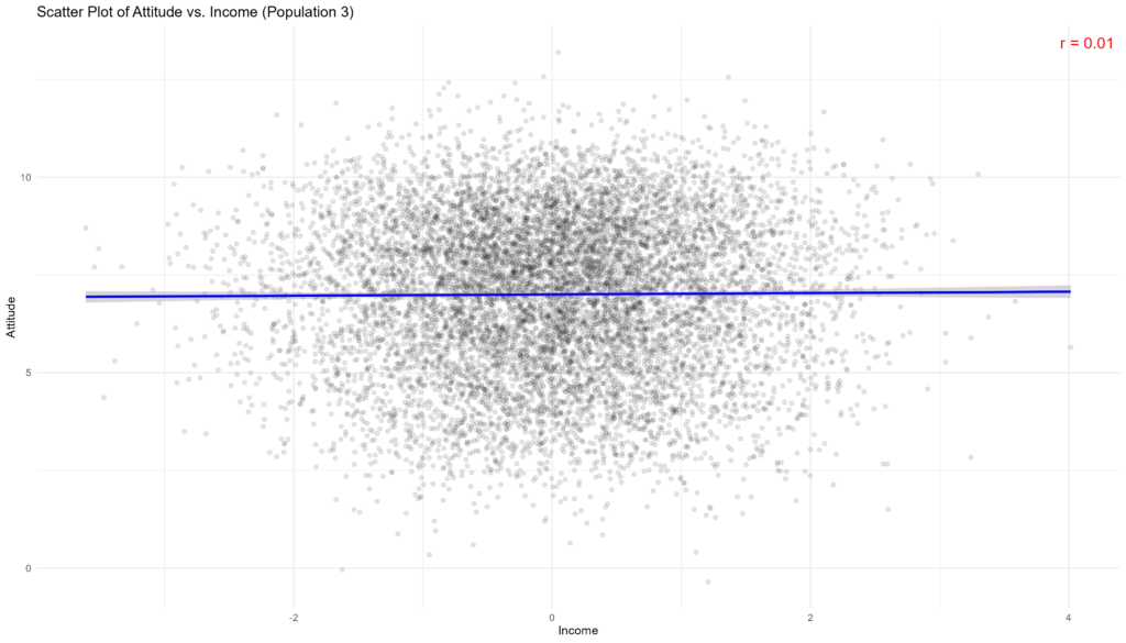
- 5 Simulate Population Data 3: small_area-level attitude variance uncorrelated with income.
- 6 Estimate bias and variance using the bootstrap method
- 7 Population 1: No Aggregate-Level Variance
- 8 Population 2: Aggregate-Level Variance Correlated with Income
- 9 Population 3: Aggregate-Level Variance, Uncorrelated with Income
- 10 Conclusion
Setup Simulation
The first step is to setup the environment and the simulation parameters. We want to generate realistically large but computationally manageable populations (n = 1,000,000) divided into 50 small areas (n_pref), with the intention of conducting 1,000 replications for bootstrap estimates and taking samples of 1,000 individuals each.
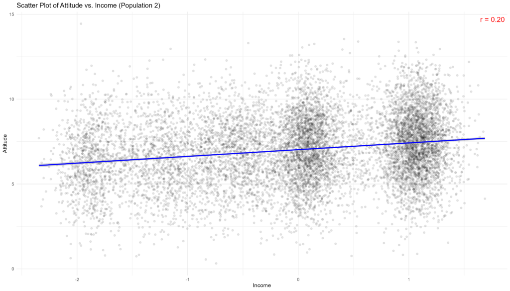
We then specify the true population parameters for the mean and standard deviation of an attitude variable with an average value of 7 and a standard deviation of 2. We also specify a correlation coefficient between the attitude and income of r = 0.2, which will be useful to generate a population for scenario 2.
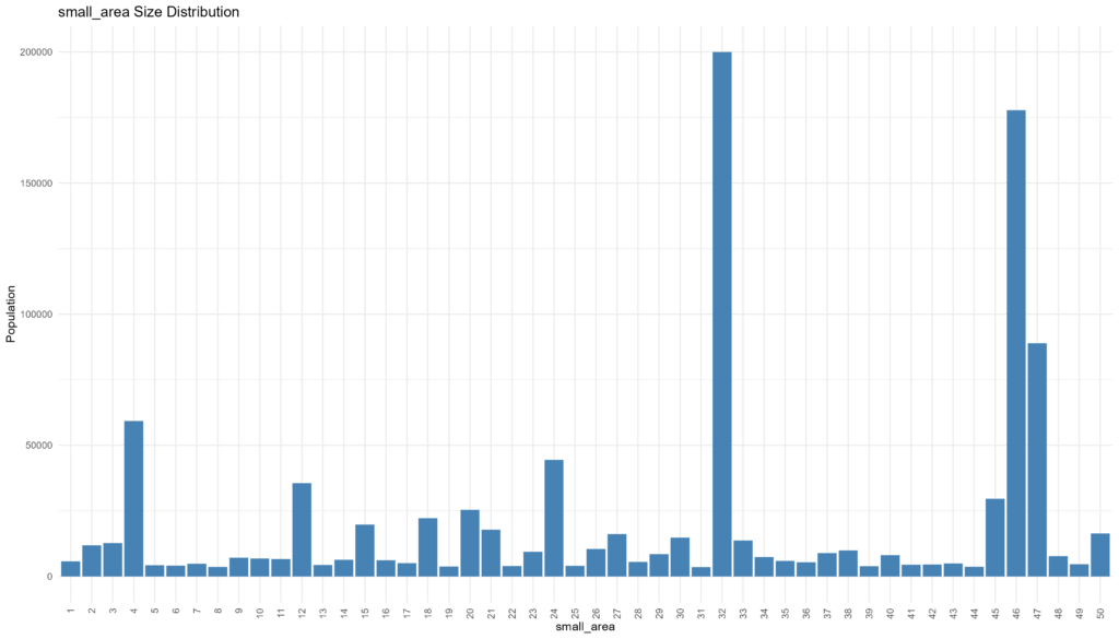
We finally generate small area sizes to approximate real-world conditions where small areas within a larger population vary significantly in size, typically following a pareto distribution or power law, and adjust the sum of these areas to match the exact total population size.
pacman::p_load(ggplot2, lme4, MASS, dplyr, lme4, rsample, purrr, tidyr)

set.seed(123) # For reproducibility
n <- 10^6 # Population size
n_pref <- 50 # Number of small_areas
n_replications <- 1000 # Number of replications for bootstrap estimates
sample_n <- 1000 # Number of samples to take

# attitude parameters

mean_attitude <- 7
sd_attitude <- 2
cor_attitude_income <- 0.2

# Generate small_area sizes with power law distribution
small_area_sizes <- round((n * 0.8) / sum(1/(1:n_pref)) * 1/(1:n_pref))
small_area_sizes <- c(small_area_sizes, n - sum(small_area_sizes))
small_area_sizes <- sample(small_area_sizes, n_pref) # Shuffle to avoid order effects

# Ensure the sum is exactly n by adjusting the last small_area
small_area_sizes[length(small_area_sizes)] <- n - sum(small_area_sizes[-length(small_area_sizes)])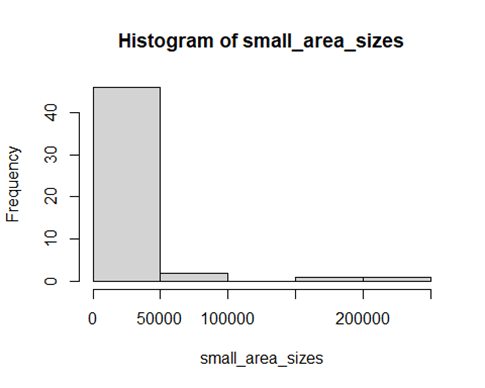
Simulation Scenarios
We then simulate three distinct population data to better determine the relative contributions of small area estimation approaches:
- Population Data 1: Simulated without small area-level variance, serving as a control scenario. All methods should perform well.
- Population Data 2: Introduced variance in attitude at the small area level, correlated with income. MRP should excel here.
- Population Data 3: Featured small area-level attitude variance not correlated with income. MRP should be similar to sample means.
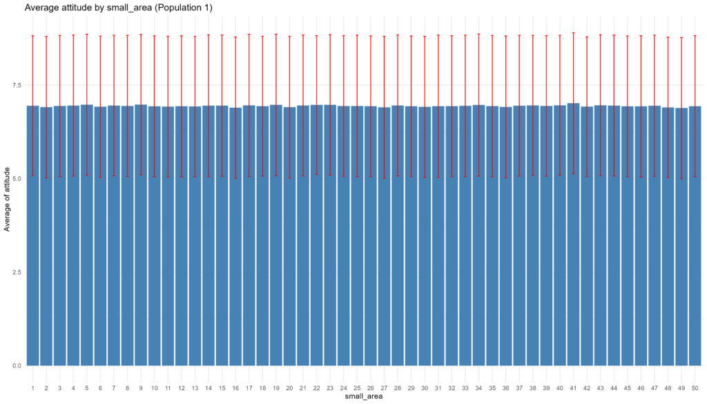
Simulate Population Data 1: No small_area-level variance
# Generate attitude/income values within each small_area  (population 1)attitude <- numeric(n)
income <- numeric(n)

for (i in 1:n_pref) {
  size_i <- small_area_sizes[i]
  attitude[small_area == i] <- pmin(10, pmax(0, rnorm(size_i, mean = mean_attitude, sd = sd_attitude)))
  income[small_area == i] <- pmin(10, pmax(0, rnorm(size_i, mean = 0, sd = 1)))
}

# Scale income (population 1)
income <- scale(income)

# Combine into a data frame
population_1 <- data.frame(small_area, attitude, income)
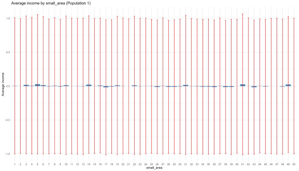
# Create "census data" of income by small_area for post-stratification

census_income <- aggregate(income ~ small_area, data = population_1, FUN = function(x) c(mean = mean(x), sd = sd(x)))
census_income$income_mean <- census_income$income[, "mean"]
census_income$income_sd <- census_income$income[, "sd"]
census_income <- census_income[, !names(census_income) %in% c("income", "income_sd")]
names(census_income)[names(census_income) == "income_mean"] <- "income"

census_income_1 <- census_income %>%
  select(small_area, income) %>%
  as_tibble()

print(census_income_1)

## # A tibble: 50 x 2
##    small_area   income
##         <int>    <dbl>
##  1          1  0.00415
##  2          2  0.00123
##  3          3  0.0187
##  4          4  0.00581
##  5          5  0.0285
##  6          6  0.0139
##  7          7 -0.00495
##  8          8  0.00589
##  9          9 -0.00668
## 10         10  0.0131
## # ... with 40 more rows
Simulate Population Data 2: small_area-level attitude variance correlated with income
# Generate income correlated with small_area number

random_noise <- rnorm(n, mean = 0, sd = 1)  # Random noise to add variability
income <- (small_area/2) + random_noise

# Ensure the overall mean of income is 0 by centering the income distribution
income <- scale(income)

# Combine into a data frame
population_2 <- data.frame(small_area, income)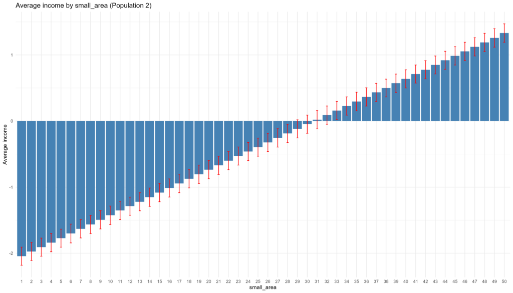
# Generate attitude with a correlation with income

income_weighted <- population_2$income * cor_attitude_income
noise <- rnorm(nrow(population_2), mean = 0, sd = 1)
population_2$attitude <- income_weighted +

# Correctly scale attitude to have a mean of 7 and a standard deviation of 2
population_2$attitude <- scale(population_2$attitude) # Scales to mean = 0, sd = 1 by default
population_2$attitude <- population_2$attitude * sd_attitude + mean_attitude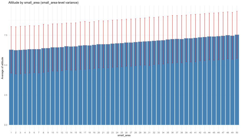
Simulate Population Data 3: small_area-level attitude variance uncorrelated with income.
# Generate income correlated with small_area number

income <- rnorm(n, mean = 0, sd = 1)  # Random noise
income <- scale(income)

# Combine into a data frame
population_3 <- data.frame(small_area, income)
# Census of income by small_area for post-stratification
census_income <- aggregate(income ~ small_area, data = population_2, FUN = function(x) c(mean = mean(x), sd = sd(x)))
census_income$income_mean <- census_income$income[, "mean"]
census_income$income_sd <- census_income$income[, "sd"]
census_income <- census_income[, !names(census_income) %in% c("income", "income_sd")]
names(census_income)[names(census_income) == "income_mean"] <- "income"
census_income_2 <- census_income %>%
select(small_area, income) %>%
as_tibble()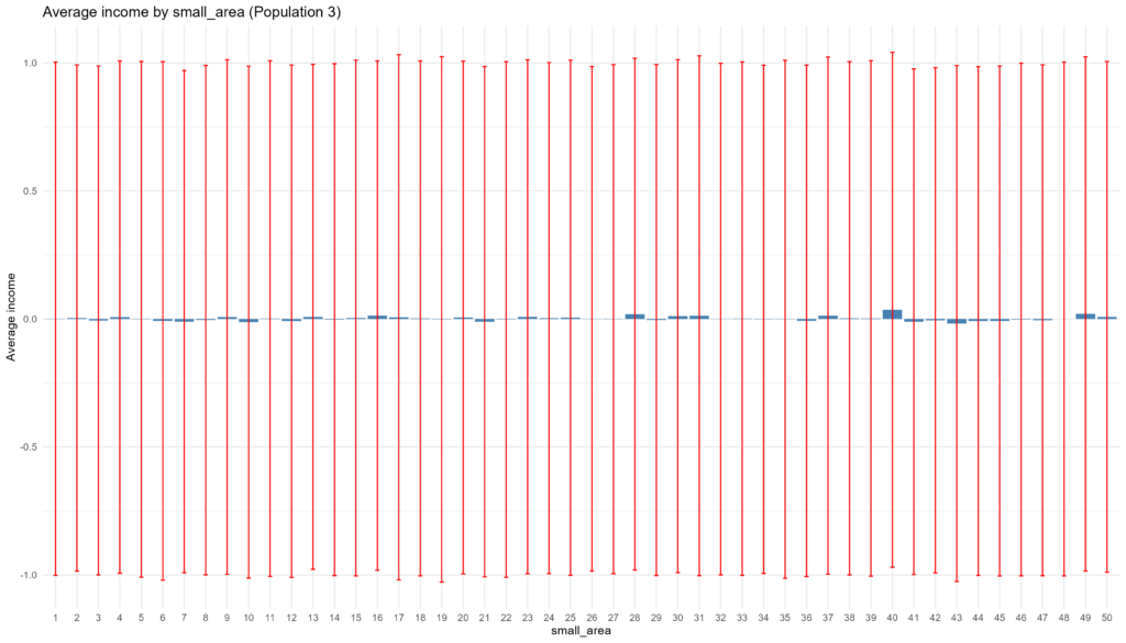
# Generate attitude with a correlation with small_area

random_noise <- rnorm(nrow(population_3), mean = 0, sd = 1)
population_3$attitude <- (small_area/10) + random_noise

# Correctly scale attitude to have a mean of 7 and a standard deviation of 2
population_3$attitude <- scale(population_3$attitude) # Scales to mean = 0, sd = 1 by default
population_3$attitude <- population_3$attitude * sd_attitude + mean_attitude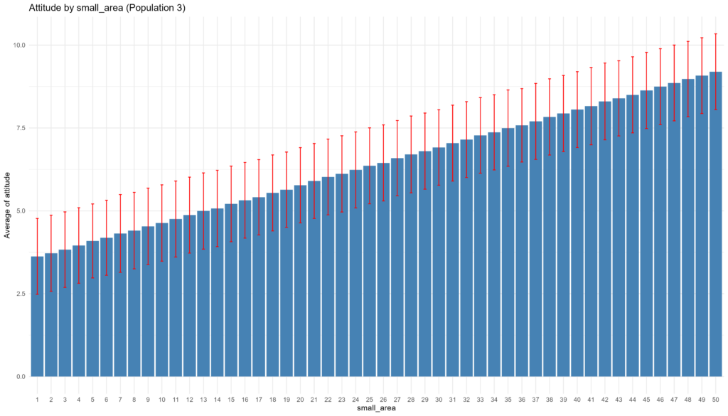
# Census of income by small_area for post-stratification

census_income <- aggregate(income ~ small_area, data = population_3, FUN = function(x) c(mean = mean(x), sd = sd(x)))
census_income$income_mean <- census_income$income[, "mean"]
census_income$income_sd <- census_income$income[, "sd"]
census_income <- census_income[, !names(census_income) %in% c("income", "income_sd")]
names(census_income)[names(census_income) == "income_mean"] <- "income"

census_income_3 <- census_income %>%
  select(small_area, income) %>%
  as_tibble()
Estimate bias and variance using the bootstrap method
Bootstrapping is a powerful statistical technique to estimate the distribution of a statistic (like the mean, variance, or median) by resampling with replacement from the original data set. Essentially, it involves taking repeated samples from the data set, computing the statistic for each sample, and then using these statistics to infer the shape of the distribution of the statistic across all possible samples from the population. This method is particularly useful when the theoretical distribution of the statistic is unknown or difficult to derive, allowing for estimation of confidence intervals, variance, and other statistical measures directly from the data without heavily relying on assumptions about its distribution.
Using the bootstrap to estimate the variance of MRP is effective because it allows for the simulation of numerous resampling processes from the original data without making strict assumptions about the data distribution.
Function to draw sample with a minimum of 10 per small_area
First we define a function to sample individuals from a dataset while ensuring a minimum representation from each small area. Initially, it guarantees that at least 10 individuals are sampled from each small area, using replacement if necessary, to meet this minimum requirement, then sampling at random, or what’s the same, with probability proportional to small area size. A
This step is added to enable calculation of means and variances using all three methods, i.e. unless we have some minimum sample size for each small area, we would not be able to use the “sample means” method to estimate the average attitude for each small area (though “fixed means” and MRP would).
sample_population_small_area <- function(data) {
# Sample a minimum of 10 from each small_area
sampled_population_1 <- data %>%
group_by(small_area) %>%
slice_sample(n = 10, replace = TRUE) %>%
ungroup()
# Calculate remaining sample size after ensuring minimum samples per small_area
remaining_sample_size <- sample_n - (n_pref * 10)
# If remaining sample size is less than 0, adjust it to 0
remaining_sample_size <- max(remaining_sample_size, 0)
# Sample the remainder from the entire dataset
sampled_population_2 <- sample_n(data, remaining_sample_size)
# Combine the two samples
sampled_data <- rbind(sampled_population_2,sampled_population_1)return(sampled_data)
}
Small Area Estimators
We then create one function for each of the proposed small area estimators using the bootstrap method.
1. `fixed_means`: This function creates a data frame (using `tibble`) with two columns: `small_area`, which is simply a sequence of numbers from 1 to `n_pref` (indicating the number of small areas), and `mean_attitude`, where each small area is assigned the same mean attitude value (`mean_attitude` variable). This function essentially sets up a baseline where all small areas have the same fixed mean attitude for comparison or further analysis.
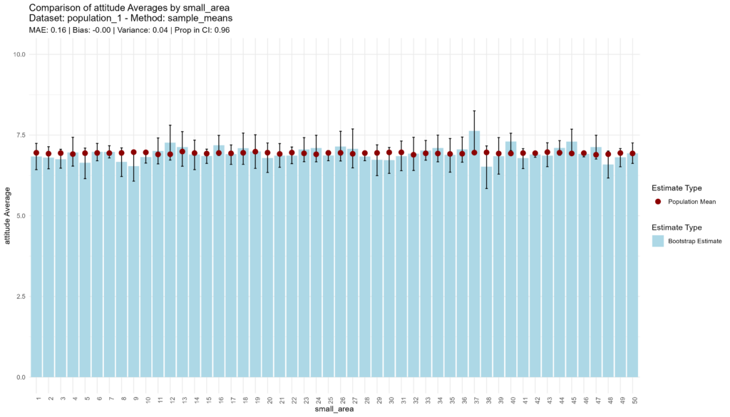
2. `sample_means`: It performs a bootstrap sampling process on the given data, sampling with replacement within each small area to maintain the same size as the original data. After sampling, it calculates the mean attitude for each small area from this bootstrap sample. This function is used to estimate the variability in mean attitudes across small areas using bootstrap samples, which can help assess the stability of these estimates or simulate sampling distributions.
3. `mrp`: This function is at the heart of applying the MRP technique. It starts by creating a bootstrap sample of the data, similar to `sample_means`. Then, it fits a multilevel (hierarchical) linear regression model (`lmer`) to this sample, predicting attitudes based on income and varying intercepts for each small area. Using this model, it predicts mean attitudes for small areas represented in a `census` data frame, adjusting predictions to remain within realistic bounds (0 to 10). This approach allows for the estimation of attitudes across small areas, adjusted for income and the specific variance within each area, which is central to MRP’s goal of providing detailed estimates even in areas where direct survey data might be sparse.
fixed_means <- function(data) {
  means <- tibble(small_area = 1:n_pref, mean_attitude = rep(mean_attitude, n_pref))
  return(means)
}

sample_means <- function(data) {
  bootstrap_sample <- data %>%
    group_by(small_area) %>%
    sample_frac(size = 1, replace = TRUE) %>%
    ungroup()
  means <- bootstrap_sample %>%
    group_by(small_area) %>%
    summarise(mean_attitude = mean(attitude, na.rm = TRUE))
  return(means)
}

mrp <- function(data, census) {
  bootstrap_sample <- data %>%
    group_by(small_area) %>%
    sample_frac(size = 1, replace = TRUE) %>%
    ungroup()
  model <- suppressMessages(lmer(attitude ~ income + (1 | small_area), data = bootstrap_sample))
  census$mean_attitude <- predict(model, newdata = census, re.form = NULL)
  means <- census %>%
    select(small_area, mean_attitude) %>%
    mutate(mean_attitude = ifelse(mean_attitude > 10, 10, ifelse(mean_attitude < 0, 0, mean_attitude))) ### Added bounds to avoid values >10 or <0
  return (means)
}
Bootstrap function to replicate mean estimations
We next define a `bootstrap_and_plot` function designed to evaluate and visualize the performance of statistical estimation methods. The function first draws a sample from the population, then performs bootstrap replications for a specified estimation method. After bootstrapping, it aggregates the results to calculate mean estimates, confidence intervals (CIs) for each small area using the percentile method, and merges these with the actual population means for direct comparison. The following performance metrics are generated for each plot.
- Accuracy: mean absolute error (MAE).
- Bias: average prediction error.
- Confidence: proportion of estimates where the true population value falls within the computed confidence intervals.
- Variance of the confidence interval across small areas .
bootstrap_and_plot <- function(population, method_function, census=NA, n_replications = 1000) {

  # Capture the names of the dataset and method function
  dataset_name <- deparse(substitute(population))
  method_name <- deparse(substitute(method_function))

  data <- sample_population_small_area(population)

  # Bootstrap estimates
  start_time <- Sys.time()

  if (method_name %in% c("mrp", "lmp")) {
    replicated_means <- replicate(n_replications, method_function(data, census), simplify = FALSE)
  } else {
    replicated_means <- replicate(n_replications, method_function(data), simplify = FALSE)
  }

  duration <- round(difftime(Sys.time(), start_time, units = "secs"))
  print(paste("Execution time:", duration, "seconds."))

  # Combine all replicate means into one dataframe
  all_means <- bind_rows(replicated_means, .id = "replicate")

  # Calculate the overall mean and confidence intervals by small_area
  final_estimates <- all_means %>%
    group_by(small_area) %>%
    summarise(estimate_mean = mean(mean_attitude),
              lower_ci = quantile(mean_attitude, probs = 0.025),
              upper_ci = quantile(mean_attitude, probs = 0.975))

  # Calculate population averages for attitude by small_area in the original population
  population_averages <- population %>%
    group_by(small_area) %>%
    summarise(population_mean = mean(attitude))

  # Merge the population averages with the sampled estimates
  comparison_data <- final_estimates %>%
    inner_join(population_averages, by = "small_area") %>%
    mutate(error = estimate_mean - population_mean)

  # Calculate the proportion of small_areas where the confidence interval includes the population mean

  comparison_data <- comparison_data %>%
    mutate(in_ci = population_mean >= lower_ci & population_mean <= upper_ci)

  proportion_in_ci <- mean(comparison_data$in_ci)

  # Calculate MAE and Bias
  mae <- mean(abs(comparison_data$error))
  bias <- mean(comparison_data$error)

  # Calculate average variance across small_areas

  average_variance <- all_means %>%
    group_by(small_area) %>%
    summarise(variance = var(mean_attitude)) %>%
    summarise(average_variance = mean(variance))

  # Plotting

  plot <- ggplot(comparison_data, aes(x = as.factor(small_area))) +
    geom_bar(aes(y = estimate_mean, fill = "Bootstrap Estimate"), stat = "identity", position = "dodge") +
    geom_errorbar(aes(ymin = lower_ci, ymax = upper_ci), width = 0.2, position = position_dodge(width = 0.9)) +
    geom_point(aes(y = population_mean, color = "Population Mean"), position = position_dodge(width = 0.9), size = 3) +
    theme_minimal() +
    labs(title = paste("Comparison of attitude Averages by small_area", "\nDataset:", dataset_name, "- Method:", method_name),
         subtitle = sprintf("MAE: %.2f | Bias: %.2f | Variance: %.2f | Prop in CI: %.2f", mae, bias, average_variance, proportion_in_ci),
         x = "small_area",
         y = "attitude Average") +
    theme(axis.text.x = element_text(angle = 90, hjust = 1)) +
    scale_fill_manual(name = "Estimate Type", values = c("Bootstrap Estimate" = "lightblue")) +
    scale_color_manual(name = "Estimate Type", values = c("Population Mean" = "darkred")) +
    ylim(0, 10)

  print(plot)

  # Define the file name
  file_name <- paste0("plot_", gsub(" ", "_", dataset_name), "_", gsub(" ", "_", method_name), ".png")

  # Save the plot
  ggsave(file_name, plot, width = 14, height = 8, units = "in")
}
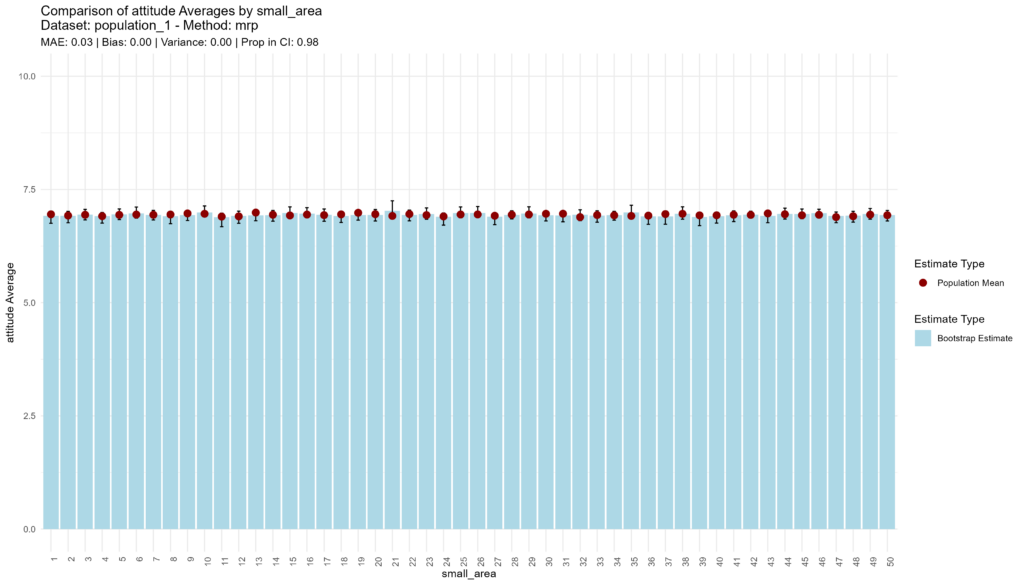
In the first population, the “fixed means” approach performs extremely well. Even if there is a significant amount of individual-level variance, since there is no variance at the aggregate level, simply imputing the mean is effective. However, since the method does not produce any variance, it does not have a confidence interval, hence 0% of the true population values fall within the estimated confidence interval. In summary, a high accuracy, low bias, low variance, but overconfident model.
bootstrap_and_plot(population=population_1, method_function=fixed_means)
## [1] "Execution time: 1 seconds."##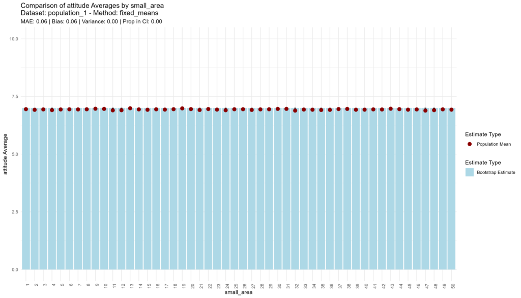
The sample means approach performs as expected, with medium accuracy, low bias, somewhat higher variance, and adequate confidence, as shown by the fact that 96% of the true population values are captured by the 95% CI. Given the CI’s are calculated using the bootstrap approach, computation time is significant (51 seconds).
bootstrap_and_plot(population=population_1, method_function=sample_means)
## [1] "Execution time: 51 seconds."
The MRP approach performs extremely well, with high accuracy, low bias, low higher variance, and adequate confidence, as shown by the fact that 98% of the true population values are captured by the 95% confidence interval. Given estimation involves multi-level regression with post-stratification and the CI’s are calculated using the bootstrap approach, computation time even higher (75 seconds) than for the sample means approach.
bootstrap_and_plot(population=population_1, method_function=mrp, census = census_income_1)## [1] "Execution time: 75 seconds."
Population 2: Aggregate-Level Variance Correlated with Income
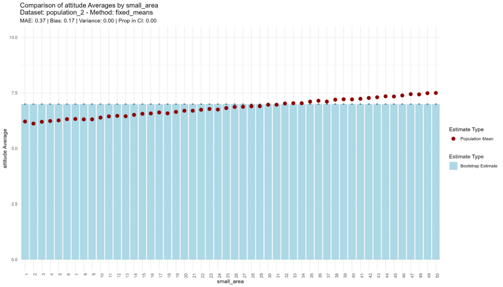
In the second population, the “fixed means” approach begins to show its colors, with low accuracy, high bias, low variance, and extreme overconfidence. But hey, at least it’s quick!
bootstrap_and_plot(population=population_2, method_function=fixed_means)
## [1] "Execution time: 1 seconds."
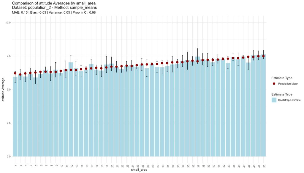
The sample means approach continues with its vanilla performance, with medium accuracy, low bias, somewhat higher variance, and adequate confidence.
bootstrap_and_plot(population=population_2, method_function=sample_means)
## [1] "Execution time: 47 seconds."
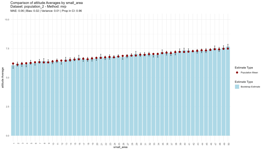
MRP again outperforms the other methods, with high accuracy, low bias, low higher variance, and adequate confidence.
bootstrap_and_plot(population=population_2, method_function=mrp, census = census_income_2)## [1] "Execution time: 76 seconds."
Population 3: Aggregate-Level Variance, Uncorrelated with Income
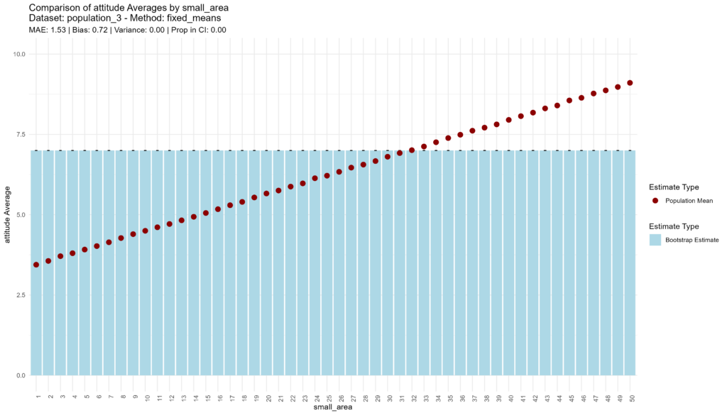
In the third population, the “fixed means” approach fails miserably, as one might expect, with very low accuracy, extremely high bias, no variance, and extreme overconfidence.
bootstrap_and_plot(population=population_3, method_function=fixed_means)
## [1] "Execution time: 1 seconds."
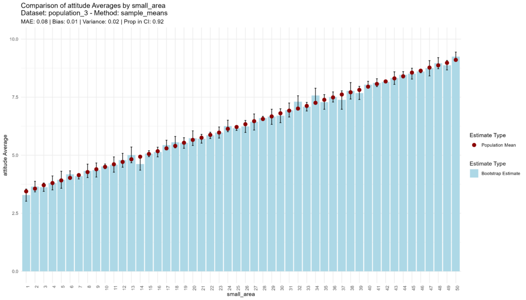
The sample means approach does not impress, neither disappoint, with medium accuracy, low bias, low variance, and adequate confidence.
bootstrap_and_plot(population=population_3, method_function=sample_means)
## [1] "Execution time: 49 seconds."
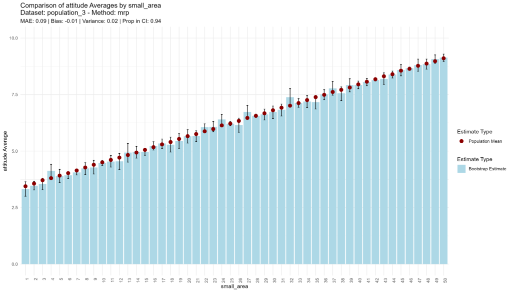
Given that income is uncorrelated with attitudes in this population, the MRP model essentially does not have any information to work with other than the small area intercepts, and so its performance is equivalent to the sample means approach (even though it takes about 24 seconds longer).
bootstrap_and_plot(population=population_3, method_function=mrp, census = census_income_3)
## [1] "Execution time: 73 seconds."
Conclusion
In summary, MRP is, at worst, equivalent to estimating small area attitudes using sample means. Where auxiliary data are available to predict outcomes, either at the individual or small area level, MRP vastly outperforms sample means.
Quite a fine and dandy performance, MRP!

Obviously this is only a toy model to serve as a proof of concept. Actual applications of MRP are much more complex, potentially involving multiple predictors at the individual and aggregate levels, random coefficients and cross-level interactions and multiple postratification cells within each small area. So please handle with care and check with an expert!