Our adventurous clients often go on daring survey missions to collect data in remote locations, armed with GPS devices to collect latitude and longitude coordinates, pinpointing the exact spots where face-to-face interviews go down. Awesome, right? Yes, but danger lurks in the shadows – the risk of re-identification! Fear not, fellow explorers, for we have the ultimate solution to save the day! Jitter it!

This post will show how to minimize this risk by displacing coordinates using the geographic displacement procedures developed by our friends at ICF International for the DHS project. This procedure aims to balance the need to protect respondent confidentiality with the need to make available to the public analytically useful data.
The procedure involves randomly displacing the GPS latitude/longitude positions for all surveys randomly, so that:
- Urban clusters have a minimum of 0 and a maximum of 2 kilometers of error.
- Rural clusters have a minimum of 0 and a maximum of 5 kilometers of positional error with a further 1% of the rural clusters displaced a minimum of 0 and a maximum of 10 kilometers.
- Setup environment:
The code begins by loading necessary R packages using the pacman package management tool. It imports various packages such as dplyr, maps, ggplot2, spatstat, and others that are required for data manipulation, visualization, and spatial operations.
if (!require("pacman")) install.packages("pacman")
library ("pacman")
pacman::p_load(dplyr, maps, ggplot2, maptools, raster, rgdal, mapproj,
spatstat, rgeos, splancs, fields, geosphere, tibble, labelled, rmarkdown)
- Generate random data within Ghana:
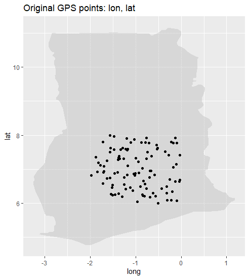
We then generate a random GPS dataset with longitude and latitude coordinates to demonstrate the procedure. For the sake of this demonstration, we select Ghana. The code below creates a dataframe named mydata with columns for latitude and longitude. The runif() function is used to generate random values for latitude and longitude within specified ranges.
n <- 100
set.seed(123)
lat <- runif(n, min = 6, max = 8)
lon <- runif(n, min = -2, max = 0)
mydata <- as.data.frame(cbind(lat, lon))
- Merge displaced GPS into the dataset:
We are now ready to create our first function to merge displaced GPS coordinates into the original dataset. The displace.merger() function takes the displaced GPS object and the column names for latitude and longitude as input. The function creates a new dataframe named mydata.displaced that combines the original dataset and the displaced GPS coordinates. It replaces the original latitude and longitude columns with the displaced values.
displace.merger <- function (displacedGPS, gps.vars) {
displaced.df <- data.frame(coordinates(displacedGPS))
row.names(displaced.df) <- which(complete.cases(mydata[,gps.vars]))
mostattributes(displaced.df$coords.x1) <- attributes(mydata[,gps.vars[1], drop=T])
mostattributes(displaced.df$coords.x2) <- attributes(mydata[,gps.vars[1], drop=T])
mydata.displaced <- left_join(rownames_to_column(mydata),
rownames_to_column(displaced.df),
by = ("rowname"))
mydata.displaced[,gps.vars] <- mydata.displaced[,c("coords.x1", "coords.x2")]
mydata.displaced <- mydata.displaced[!names(mydata.displaced) %in% c("rowname",
"coords.x1",
"coords.x2")]
return (mydata.displaced)
}
- Geographic displacement procedure based on DHS policy
We next create our workhorse gps displacement function. The displace() function is defined to perform the geographic displacement procedure. It takes the column names for latitude and longitude, administrative boundaries data (admin), the number of samples to generate (samp_num), and the number of points to randomly generate around each GPS coordinate (other_num). The function begins by plotting the original GPS points on a map. It then proceeds to perform the displacement procedure using a series of steps including buffering, intersection with administrative boundaries, and generating random points. The resulting displaced GPS points are merged into the original dataset using the displace.merger() function. The function also includes additional map plots to visualize the displaced GPS points. Finally, it returns the displaced dataset. This function is essentially an adaptation to R from the original Python code from Brendan Collis (Blue Raster) and released by DHS: https://dhsprogram.com/pubs/pdf/SAR7/SAR7.pdf.
The function is a bit lengthy so we are not going to post it here, but you can find it in our Github.
- Load Goespatial datafiles
We now load the necessary map data using the map_data() function. We specifically filter the data to focus on Ghana by specifying the region as “Ghana”. Next, we obtain the administrative boundaries data for Ghana. In the commented line of code, there is an alternative method using the raster::getData() function, which allows you to retrieve the country map based on the standard 2-letter country codes directly from the UC Davis server. However be advised that this server is often down, so we like to download the .rds file and then source it locally using the readRDS() function to read the administrative boundaries data directly from a file named “gadm36_GHA_0_sp.rds”. This file contains spatial information for the national boundaries of Ghana, and is used by the displace() function to ensure that jittered points don’t go beyond the national boundaries. This procedure can be specified at lower administrative levels if necessary by downloading the requisite .rds file.
countrymap <- map_data("world") %>% filter(region=="Ghana")  #!!! Select correct country
#admin <- raster::getData("GADM", country="GH", level=0) #!!! Select correct country map using standard 2-letter country codes: https://en.wikipedia.org/wiki/ISO_3166-1_alpha-2
admin <- readRDS(file="gadm36_GHA_0_sp.rds")
- Run displacement procedure
Finally, we specify the relevant variables by creating a vector named gps.vars with the column names “lon” and “lat”. It’s important to keep in mind that longitude should always come first, followed by latitude. We then call the displace() function, passing the gps.vars vector, along with other arguments. The displace() function performs a geographic displacement procedure on the GPS data. It takes the administrative boundaries data, stored in the admin variable, as well as the number of samples to generate (samp_num) and the number of points to randomly generate around each GPS coordinate (other_num).
Executing this code may take a few minutes to complete, as the displacement procedure involves multiple steps. It processes the GPS data and generates a new dataset named mydata with the displaced GPS points.
gps.vars <- c("lon", "lat") # !!!Include relevant variables, always longitude first, latitude second.
mydata <- displace(gps.vars, admin=admin, samp_num=1, other_num=100000) # May take a few minutes to process.
[1] “Summary Long/Lat statistics before displacement”
lon lat
Min. :-1.97907 Min. :6.001
1st Qu.:-1.38781 1st Qu.:6.491
Median :-1.00017 Median :6.933
Mean :-0.97155 Mean :6.997
3rd Qu.:-0.57727 3rd Qu.:7.511
Max. :-0.02872 Max. :7.989
The displaced GPS points are shown below in red, with their original location in black.
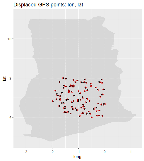
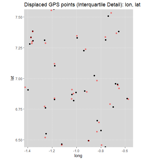
A closer detail is shown below. As you can see, the displacement is relatively minor, preserving most of the analytical advantages of the GPS data, while introducing enough uncertainty in the original location of the interview to minimize the risk of re-identification.
“Summary Long/Lat statistics after displacement”
lon lat
Min. :-1.98104 Min. :5.995
1st Qu.:-1.40776 1st Qu.:6.506
Median :-1.01086 Median :6.926
Mean :-0.97139 Mean :6.996
3rd Qu.:-0.56935 3rd Qu.:7.524
Max. : 0.01255 Max. :8.003
“Processing time = 59 seconds”
So remember, when dealing with GPS data along with other sensitive information, better jitter it! This procedure can be useful in various applications where preserving the confidentiality of geospatial data is necessary.
Please note that the code provided in the blog post might require additional modifications or refinements depending on specific use cases and data requirements. It is always recommended to carefully review and adapt the code to fit your specific needs.